Preamble

R packages

The required R packages are explicitly listed here.

library(raster)
library(forcats)
library(ggmap)
library(lme4)
library(nlme)
library(pander)
library(haven)
library(knitr)
library(fields)
library(rgdal)
library(sf)
library(randomForest)
library(tidyverse)

Introduction

To meet the high demand on the geographic dis-aggregation of key indicators, UNFPA Small Area Estimation (SAE) work has initially focused on the combination of census data and survey data. But to be rigorously valid, one necessary condition is that both the survey and the census should be carried out at the same moment so that the distributions of the variables from the survey converge toward their census counterpart. But in the real world, the census is generally “old” and the survey data contemporaneous. In this more frequent situation, the method suffers from different biases that have been pointed out by numerous authors (Tarozzi & Deaton, 2009; Molina & Rao 2010; Nguyen, 2012). So a new SAE approach needs to be developed for the countries without recent census data available. This document describes a method that fills this gap by relying only on the survey Data and borrowing strength from the spatial correlation within the sample.

This document describes the detailed steps for unit level model small area estimation. Each step is accompanied with the associated R code, followed by the detailed description for the code. The Ghana DHS data is taken as the example.

`unsae` package

Modeling requires an R package called unsae available on here.
The development of unsae package has been complete, yet documentation may not be fully provided.
To install unsae, run the following code:

devtools::install_github("ydhwang/unsae")

Then it can be loaded by running:

library(unsae)

In case the software returns that it could when seeing the could not find function error messages or something similar, it means the package may have been updated. So you need to run the devtools::install_github("ydhwang/unsae") again

Data preparation

Description

This section illustrates the data preparation steps for the unit level model.
Throughout, we assume that the data files are stored in ../data/ (locations are all relative).
Alternatively, one can use file.choose() and locate the file manually.

DHS Data loading

Detailed description of DHS data can be found at DHS site.
DHS data files are assumed to be stored in ../data/2011 DHS/.
For Ghana case,
- GHHR72FL.SAV: individual data
- GHIR72FL.SAV: Household data
We use haven::read_sav function to read the data files stored in SAV format.

Individual level data handling

Artifact of converting SPSS SAV file to “flattened” data table form can be removed by choosing the variables that don’t have “$” in their names.
They are excluded from the analysis. In the code, it looks for $ string and excludes them from the data set.

Multiple occurrence variables are placed one after the other by occurrence; all variables for occurrence 1 precede all variables for occurrence 2 and so on; multiple occurrence variables have a numeric sub- index that indicate the occurrence number.

Selection of the variables (1)

Some information can be difficult to use, so removed from the analysis.
V003 is the Respondent’s line number in the household schedule, so removed from the analysis.

indiv_ini <- read_sav("sae-geospatial/data/2011 DHS/GHIR72FL.SAV")   
indiv <- indiv_ini %>% select(!matches("[\\$]")) %>% 
  select(-V000) %>% # same country 
  select(-V003)

Selection of the variables (2)

indiv <- indiv %>% select_if(function(x) mean(is.na(x)) < 0.3)

For the purpose of SAE, the variables with too high missing rate are not useful. Hence we exclude those with less than 30 % missing.
We can see that 4079 columns are reduced to 405.
It’s important to notice that in the real world, one should handle the missing variable problem one-by-one.

Glimpse of the data

We can see the variable information here presented in Table label.
Only first few are presented here.

info <- lapply(indiv, function(x) attr(x, "label"))
ind_var_tbl <- tibble(COL = names(info), DESC = as.character(info)) 
ind_var_tbl %>% head %>% pander

COL	DESC
CASEID	Case Identification
V001	Cluster number
V002	Household number
V004	Ultimate area unit
V005	Women’s individual sample weight (6 decimals)
V006	Month of interview

Household level

We first conduct the data cleaning for household data in a similar manner.

household_ini <- read_sav("sae-geospatial/data/2011 DHS/GHHR72FL.SAV")
household <- household_ini %>% select(!matches("[\\$]"))

Renaming

household <- household %>% 
  rename(V000 = HV000, V001 = HV001, V002 = HV002, V003 = HV003, V004 = HV004)

The matching key information can be found in HV000, HV001, HV0002, HV003, HV004. They are renamed to be used for joining with the individual data table.

HV000 Country code and phase
HV001 Cluster number
HV002 Household number
HV003 Respondent’s line number (answering Household questionnaire)
HV004 Ultimate area unit

Selection of the variables (3)

household <- household %>% select_if(function(x) mean(is.na(x)) < 0.3) %>% select(-V000) %>% 
  select(-V003) # same country

Same missing rules are applied to select the relevant variables. We can see that 3028 columns are reduced to 142.

Glimpse of the data

Similarly to the individual data, only first few are presented here.

info <- lapply(household, function(x) attr(x, "label"))
house_var_tbl <- tibble(COL = names(info), DESC = as.character(info)) 
house_var_tbl %>% head %>% pander

COL	DESC
HHID	Case Identification
V001	Cluster number
V002	Household number
V004	Ultimate area unit
HV005	Household sample weight (6 decimals)
HV006	Month of interview

Joining the individual and household data

We combine the individual data set and household data to create dhs_expanded.
We join the individual and household data sets by using V000, V001, V0002, V003, V004 as key variables.

dhs_expanded <- left_join(indiv, household, by = c("V001", "V002", "V004")) %>% 
  arrange(V001)

HV004: Ultimate area unit is a number assigned to each sample point to identify the ultimate area units used in the collection of data. This variable is usually the same as the cluster number, but may be a sequentially numbered variable for samples with a more complicated structure.

Data modification

V218 Number of living children; convert it into three categories and rename it as V218R
V013: Age in 5-year groups; convert it into three categories and rename it as V013R

V218R
         0        1-2        3-4 5 and more 
         0          1          3          5 

V013R
15-24 25-34 35-49 
    1     2     3

Conversion

The age group variables are re-coded into a fewer categories.

dhs_expanded <- dhs_expanded %>% mutate(V013R = 
                         ifelse(V013 %in% 1:2, 1, 
                                ifelse(V013 %in% 3:4, 2, 
                                       ifelse(V013 > 4, 3, V013))))

dhs_expanded <- dhs_expanded %>% 
  mutate(V218R = 
           ifelse(V218 == 0, 0, ifelse(V218 == 1|V218 == 2, 1, 
                                       ifelse(V218 ==3|V218 ==4, 3, 
                                              ifelse(V218 >=5, 5, V218)))))

dhs_expanded <- dhs_expanded %>% select_if(function(x) mean(is.na(x)) < 0.9) # remove if more than 10% missing

Additional steps followed to remove columns with too much missing info.

Defining the target variables

Contraceptive prevalence rate (CPR) - using V313: combine 1, 2, 3 as “Yes”; 0 as “No.
Modern contraceptive prevalence rate (CPRm) - using V313: combine 0, 1, 2, 3 as “No”; 3 as “Yes”.
Unmet need for family planning rate (UNR) - using V626: combining 1, 2 as “Yes” (unmet need for family planning); combining all other answers as “No”.

dhs_reduced <- 
dhs_expanded %>% 
  select(V013R, V106, V218R, V025, V120, V127, V128, V128, V129, V113, 
         V001, V005, # survey info part
                   V119,
                   HV206, 
                   V130, 
                   V116,
                   V151,
                   V150, 
                   V626, V313) %>% 
  mutate(CPR = ifelse(V313 == 0, 0, 1)) %>% 
  mutate(CPRm = ifelse(V313 == 3, "Yes", "No")) %>% 
  mutate(UNR = ifelse(V626 == 1|V626 == 2, "Yes", "No")) %>% 
  select(-V313, -V626)

dhs_reduced  <- dhs_reduced %>% 
  mutate_all(as_factor) %>% 
  mutate(V218R = ifelse(V218R == "5 and more"|V218R == "3-4",
                        "3 or more", V218R)) 

attr(dhs_reduced$V218R, "label") <- attr(dhs_expanded$V218, "label")

Quick screeing of key variables

This step is quickly screen the important variables found based on a machine learning based method.
The example below shows the case where V013R, V106, V218R, V025, V120, V127, V128, V128, V129, V113, V119, HV206, V130, V116, V151, V150 are used as the candidates, and choose the seemingly important six variables among them.
To see the detail about the metric, see this.

temp_set <- dhs_reduced %>% na.omit
temp_rf <- randomForest(CPR ~ V013R + V106 + V218R + V025 + V120 + V127 + V128 + V128 + V129 + V113 + V119 + 
                          HV206 + V130 + V116 + V151 + V150, data = temp_set)
imp_tbl <- tibble(imp = as.numeric(importance(temp_rf)), key = rownames(importance(temp_rf))) %>% mutate(q = rank(-imp))
selected_06 <- imp_tbl %>% filter(q  <= 6) %>% arrange(-imp)
info_v <- lapply(temp_set, function(x) attr(x, "label")) %>% bind_rows %>% gather
left_join(selected_06, info_v, by = "key") %>% select(-imp) %>% pander()

key	q	value
V113	1	Source of drinking water
V130	2	Religion
V128	3	Main wall material
V116	4	Type of toilet facility
V127	5	Main floor material
V218R	6	Number of living children

Additional steps to simplify the data (1)

Many problems are caused when we carry variables with too many categories, where many categories have few counts.
fct_lump_prop combines levels that appear less than 10 % and create a new category named “Other”.

target <- selected_06$key
reduced_tbl <- 
  temp_set %>% 
  mutate_if(function(x) n_distinct(x) < 20, as.factor) %>% 
  mutate_at(all_of(target), function(x) fct_lump_prop(x, 0.1, other_level = "Other"))

Additional steps to simplify the data (2)

reduced_tbl now has columns with fewer categories after lumping levels with less than 10% proportion.
As a comparison,

temp_set %>% group_by(V130) %>% tally %>% pander

V130	n
Catholic	1341
Anglican	72
Methodist	547
Presbyterian	513
Pentecostal/charismatic	3456
Other Christian	1239
Islam	1726
Traditional/spiritualist	226
No religion	273
Other	1

reduced_tbl %>% group_by(V130) %>% tally %>% pander

V130	n
Catholic	1341
Pentecostal/charismatic	3456
Other Christian	1239
Islam	1726
Other	1632

This “lumping” process improves overall model fitting by removing the (near-) singularity of the model matrix.
The model selection step is automated in the code below.

Automatic Model fitting

# automation of this needs a carefully examined set of the variables
fe_form <- paste(selected_06$key, collapse = " + ")
full_form <- as.formula(paste("CPR ~ ", fe_form, "+ (1|V001)"))

# full model (with all data)
model_out <- glmer(formula = full_form, data = reduced_tbl, family = binomial(link = "logit"))

We use the selected 6 variables from the screening process.
It automatically writes a formula taking CPR as our target indicator, and the survey cluster as a random effect.
To see what’s the formula, see the following output of full_form (“full” formula including fixed effects and random effect).

print(full_form)

## CPR ~ V113 + V130 + V128 + V116 + V127 + V218R + (1 | V001)

In this example, is used in glmer, generalized linear mixed effects model. Users can use this in the later part as a reference.

Spatial data loading

Spatial data preparation

We are loading the spatial part of DHS data for SAE.
In this example, we use the geographic information set from DHS webpage.
It is assumed to be stored in the following location:

country_shp <- st_read("sae-geospatial/data/2011 DHS/Spatial/GHGE71FL/GHGE71FL.shp", quiet = TRUE)

Important Notes

There are some occasions in which cluster coordinate information is missing in survey data.
It varies with the country, so the user needs to pay attention to the availability and other potential issues.

## handling missing coord
mis_mark <- country_shp %>% filter((LATNUM == 0 & LONGNUM ==0))
country_shp <- country_shp %>% filter(!(LATNUM == 0 & LONGNUM ==0)) %>% filter(!is.na(LATNUM))

Map image tiles downloading

bounding_box <- st_bbox(country_shp) %>% as.numeric  # getting the bounding box
country_map <- get_stamenmap(bbox = bounding_box, messaging = FALSE, zoom = 8, 
                       maptype = "toner-lite", format = c("png"))
ggmap(country_map, extent = "device")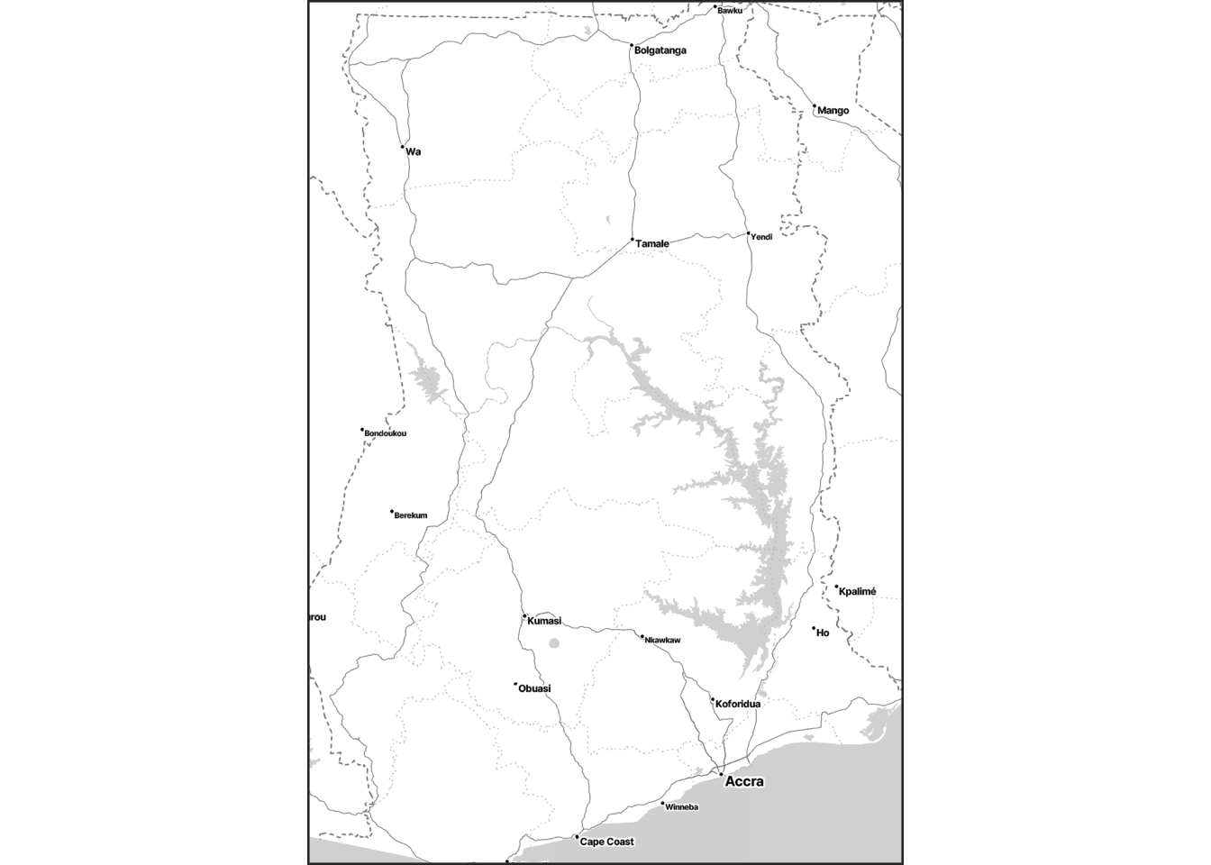

To download the map image tiles, we first need to identify the bounding box of the (country) map.
Once bounding box is found, the code below uses bounding box information to download the matching part of the image tiles.
country_map object will be used as a base layer for plotting in the remaining part.

Model fitting

Description

In this section, we will describe the detail of the model fitting process.

Cluster-wise estimate (naive)

One may consider a simple counting for each cluster.
In the reduced_tbl, DHSCLUST information was stored as V001 (see DHS webpage.)

reduced_tbl <- reduced_tbl %>%  
  rename(DHSCLUST = V001) %>% 
  mutate(DHSCLUST = as.integer(DHSCLUST))

We group the data set by DHSCLUST, and calculate the statistics for each cluster.
Depending on the needs, one may calculate the other statistics.

cluster_result <- reduced_tbl %>%  
  group_by(DHSCLUST) %>% 
  summarize(Prop_raw = mean(CPRm == "Yes"))

To see the first few clusters,

DHSCLUST	Prop_raw
1	0.03704
2	0.1429
3	0
4	0
5	0.1538
6	0.2

Removing the clusters with missing coordinates

We need to remove the clusters with missing coordinates.
Then we create the table named coord_info of the coordinate information associated with the DHS data.

valid_set <- anti_join(reduced_tbl, mis_mark, by = "DHSCLUST") 
coord_info <- tibble(DHSCLUST = country_shp$DHSCLUST, lon = country_shp$LONGNUM, lat = country_shp$LATNUM)

coord_info is a tibble with three columns – DHSCLUST, lon, lat. This tibble will be used to join the spatial coordinates to the survey data.

valid_set_with_sp <- left_join(valid_set, coord_info, by = "DHSCLUST")
valid_set_with_sp <- valid_set_with_sp %>% 
  mutate(DHSCLUST = as.factor(DHSCLUST))

valid_set_with_sp now has spatial coordinates.

Model fitting

We first consider the generalized linear mixed effects model without no spatial consideration, and store it as mod_lme.
The model, however, has cluster random effect: \[\begin{eqnarray} \eta &=& \mathbf{X} \boldsymbol{\beta} + \mathbf{Z} \mathbf{b},\\ g(\cdot) &=& \textrm{link function},\\ h(\cdot) &=& g^{-1}(\cdot) = \textrm{inverse link function}, \end{eqnarray}\] where $\mathbf{b}$ is independent cluster random effect term (with a diagonal covariance matrix, cov($\mathbf{b} = \sigma_b^2 \mathbf{I}$).

mod_lme <- 
glmer(CPR ~ 
          V218R + V013R + (1 | DHSCLUST), 
          family = binomial, 
          data = valid_set_with_sp)

Small area model fitting

Now we can use multilevel_EM, which gives a spatial model.

spatial_model_fit <- 
  multilevel_EM(formula = "CPR ~ V218R + V013R + (1 | DHSCLUST)",
                data = valid_set_with_sp, coordinates = c("lon", "lat"))

## ...EM iteration: 1 
## ...EM iteration: 2 
## ...EM iteration: 3

It needs three arguments:
- formula: (string) formula that follows glmer syntax. It only takes one random effects (cluster).
- data: name of the data set.
- coordinates: the name of coordinates within the data. These columns should exist within the data set provided.
- It often takes a while, so it prints out the number of EM iteration while it is being calculated.

Notes on `multilevel_EM`

Being different from mod_lme from glmer, multilevel_EM uses a spatial model for $\mathbf{b}$; specifically, \[ \mathbf{b} \sim N(\mathbf{0}, \mathbf{C}), \] where
$\mathbf{b}=(b_1, b_2, \cdots, b_M)'$ and $\mathbf{C}_n=(C_{ij})$ with \[ C_{ij} = \exp ( - \lambda \left\| \mathbf{s}_i - \mathbf{s}_j \right\|^2 ) + g \delta_{\mathbf{s}_i, \mathbf{s}_j}. \]
For the detail, see the accompanied technical document.

Preparing the admin shape file

raster map

Unfortunately, there is no unified data source for different countries that handles country boundary files (note: DHS shapefile is the points for the survey locations).
The example data used in this note is from here.
Alternative files like this can be used, and yet shape files from other sources are not standardized, so user needs to be careful.

What we will do:

The code below does the following.

Import the shape file.
Draw a map plot from the shape file (validation).
Extract the admin border (level 1); however the levels are not the same across different countries.
Create the grid over the country bounding box and then choose those overlapping with the country boundary.
Draw a map plot from the grid (validation).
Create grid_coord, with the coordinates assigned to each grid points.

Importing the shape files

We first import the shapefiles, and then (visually) check the data.
The shapefile contains the country border (not the small areas).

country_border <- st_read("sae-geospatial/data/shps/sdr_subnational_boundaries.shp", quiet = TRUE)
ggplot(country_border) + geom_sf()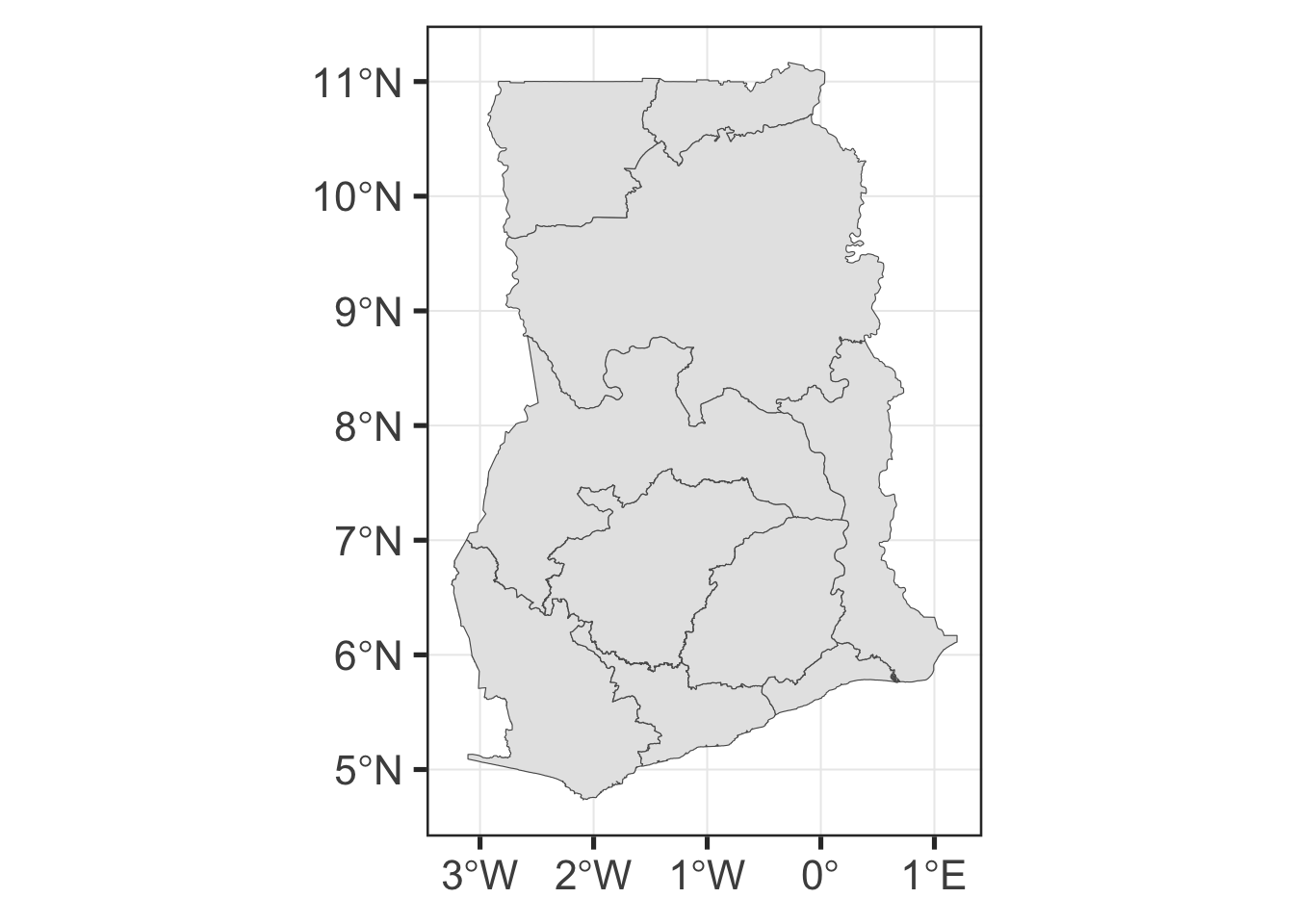

Creating a grid

Now we create a grid so that we can use as a baseline for inference.
We first create a coordinates grid as simple feature then we convert it into a tibble so that we can use it with spatial_model_fit. The tibble is named grid_coord.
Since we used lon and lat as the coordinates’ name, we need to rename X and Y to lon and lat.

grid <- country_border %>% st_make_grid(cellsize = 0.1, what = "centers") %>% st_intersection(country_border)  
ggplot() + geom_sf(data = grid)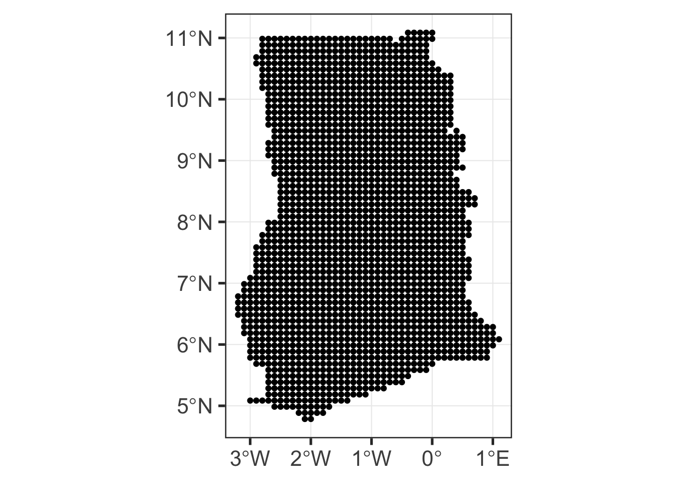

grid_coord <- st_coordinates(grid) %>% as_tibble() %>% 
  rename(lon = X, lat = Y)

Prediction based on resampling

Once grid_coord is available, the code below chooses the nearest 10% of the (survey) clusters for each grid, sample 40% of them, and make a prediction for each grid point using unit level model by treating the sampled survey as observed data.
We want to get a set of predictions for each grid in grid_coord, so for loop runs over grid_coord.
All clusters in DHS data are considered for each grid point.
Once the loop is complete, it combines into a single tibble and then indexed for every grid point – named grid_tbl.

cluster_coord <- coord_info %>% dplyr::select(lon, lat) %>% na.omit

covariates_list <- list()

for (c_i in 1:nrow(grid_coord)){
  cluster_dist_temp <- coord_info
  cluster_dist_temp$p_rank <- rdist(cluster_coord, grid_coord[c_i,]) %>% percent_rank()

  chosen_coord <- cluster_dist_temp %>% filter(p_rank <= 0.1) 
  chosen_tbl <- valid_set_with_sp %>% filter(DHSCLUST %in% chosen_coord$DHSCLUST)
  
  covariates_list[[c_i]] <-   chosen_tbl %>% sample_frac(0.4) %>% 
    select(V013R, V218R, V119, HV206)

}
grid_coord$grid_index <- 1:nrow(grid_coord) %>% as.character()
grid_samples <- bind_rows(covariates_list, .id = "grid_index")
grid_tbl <- left_join(grid_samples, grid_coord, by = "grid_index")

Creating a grid map

grid_tbl can be used to create a grid map.
When predicting at a new location (not in the DHS survey), predict_EM function is used.
predict_EM is a wrapper taking two inputs: name of the spatial model obtained from and multilevel_EM and a new data set.
New data set must have all the predictor variables used with multilevel_EM, as well as two coordinates (in this example, lon and lat).

Calculation for each grid

For each grid point, it uses the sampled survey data to make prediction.
Then it aggregates all the prediction to get the average rate for each point.

# this is grid level aggregation
# predict function 

g_index <- grid_tbl$grid_index %>% unique
grid_tbl$yhat <- NA

for (g in seq_along(g_index)){
  g_tbl <- grid_tbl %>% filter(grid_index == g_index[g])
  grid_tbl$yhat[grid_tbl$grid_index == g_index[g]] <- 
    predict_em(spatial_model_fit, test_set = g_tbl)  
}

raster_tbl <- grid_tbl %>% 
  group_by(lat, lon) %>% 
  summarise(m_yhat = mean(yhat), .groups = "drop")

Plotting

Plotting the grid points.

ggplot(raster_tbl) + aes(y = lat, x = lon, colour = m_yhat) +
  xlab("") + ylab("") +
  geom_point(size = 3, alpha = 0.5) + scale_colour_viridis_c("contraception", option = "C") + coord_map()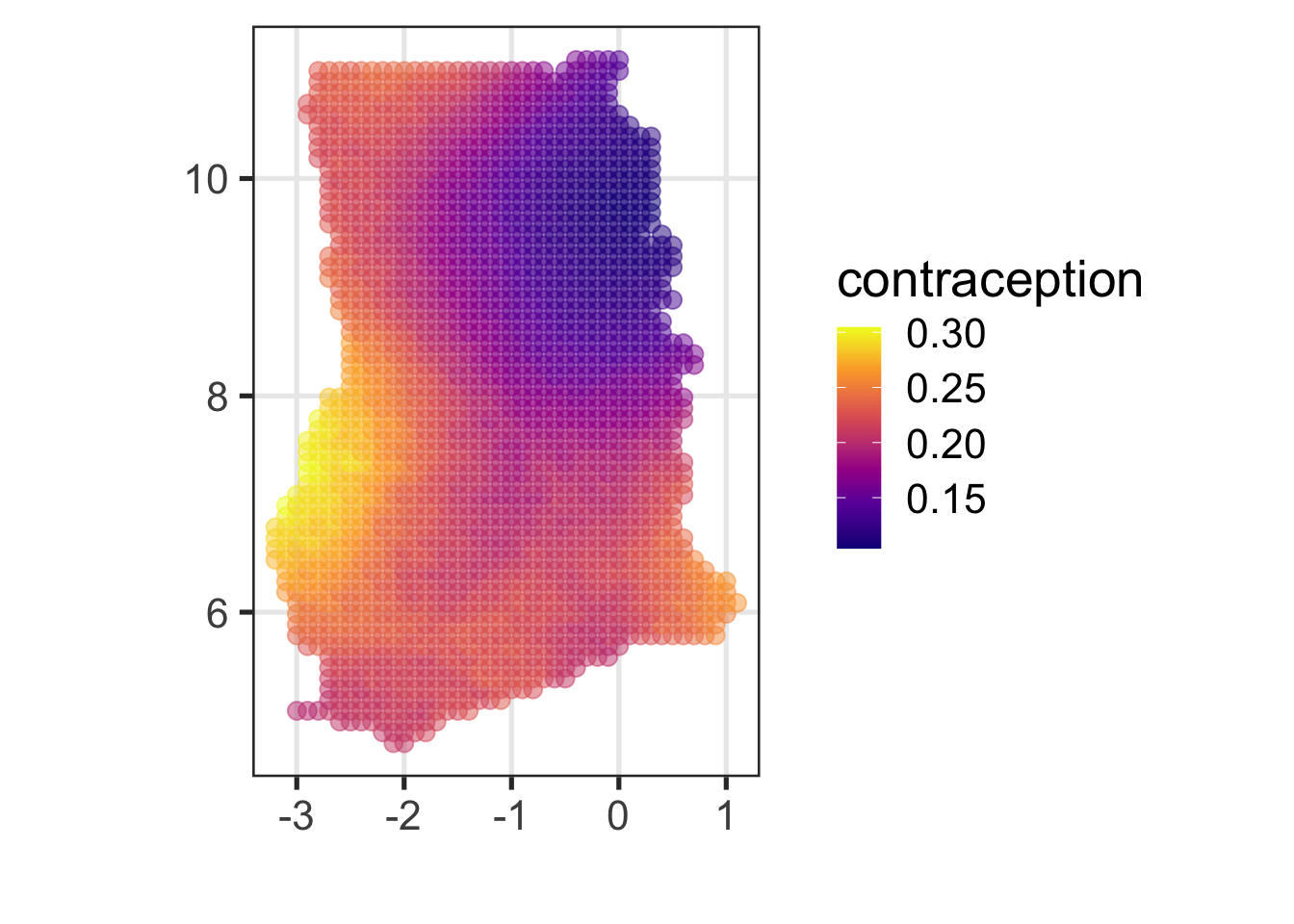

Overlaying the points over the map.

(out <-
ggmap(country_map, extent = "device")  +
  xlab("") + ylab("") +
  geom_point(data = raster_tbl, aes(y = lat, x = lon, colour = m_yhat), size = 3, alpha = 0.3) + scale_colour_viridis_c("contraception", option = "C"))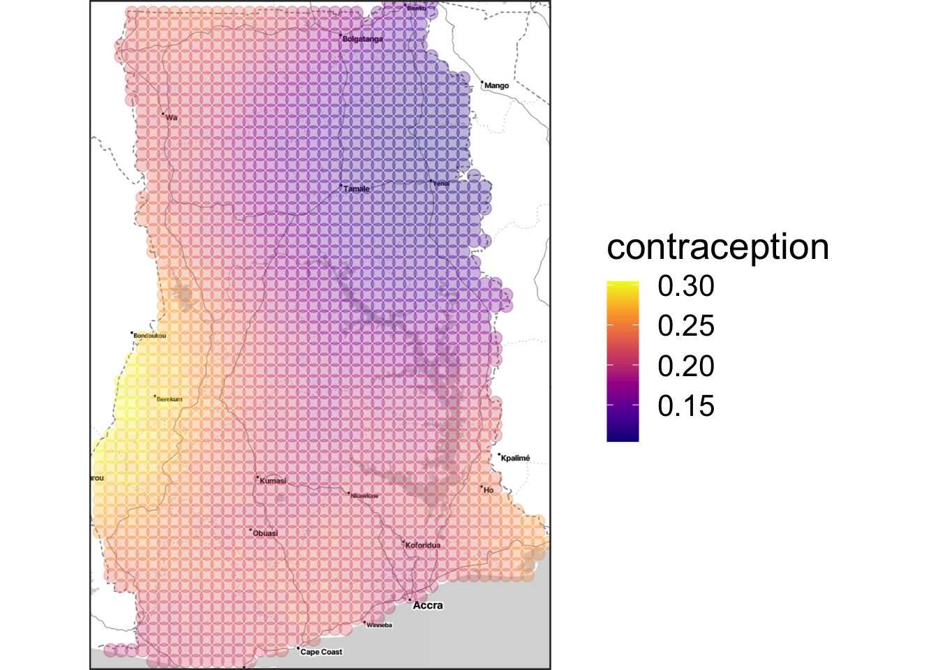

One can get the raster_map.png file by running ggsave(out, filename = "raster_map.png", width = 10, height = 8).

Area level (overview)

Now we are creating a – administrative level 2 – small area estimate map.
Shapefile is from here.
We are using the grid_coord we created from the raster map.
Now we choose the intersection of grid point with each admin area, and then take the average over it.

Importing the shapefile

We import the administrative file.
One should choose the right administrative level from the available data set.
In this example, we use level 2.

level_2_geom <- st_read("sae-geospatial/data/admin_shapefiles/gha_admbnda_adm2_gss_20210308.shp", quiet = TRUE)

Producing the prediction grid

For each area (administrative region), we create a $7\times 7$ box grid and choose the portion within the area.
For each point within the area, we choose the nearest 10% clusters (from DHS survey), and sample 30% from those clusters’ data.
Then we calculate the prediction for each point, and MSE for each area.
In this example, the model has two predictor variables V218R and V013R, which can be found in the code. If the model uses different variables, one can change the modeling part.

outcome <- 
  produce_m_v_sae(spatial_model_fit, level_2_geom, 
                  coord_info, frac = 0.1, resampling = 0.3, counter = FALSE)

Creating a plot

sae_map <- ggplot(outcome) + 
  geom_sf(aes(fill = m)) + 
  scale_fill_viridis_c(name = "Modern \nContraception Use", option = "B") 
print(sae_map)

sae_map2 <- ggplot(outcome) + 
  geom_sf(aes(fill = v)) + 
  scale_fill_viridis_c(name = "Modern \nContraception Use (MSE)", option = "B") 
print(sae_map2)

One can create the ghana_sae_map_1.png by running ggsave(sae_map, filename = "ghana_sae_map_1.png", width = 8, height = 8).

Ghana Unit Level Modeling Document

Preamble

R packages

Introduction

Introduction

unsae package

Data preparation

Description

DHS Data loading

Individual level data handling

Selection of the variables (1)

Selection of the variables (2)

Glimpse of the data

Household level

Renaming

Selection of the variables (3)

Glimpse of the data

Joining the individual and household data

Data modification

Conversion

Defining the target variables

Quick screeing of key variables

Additional steps to simplify the data (1)

Additional steps to simplify the data (2)

Automatic Model fitting

Spatial data loading

Spatial data preparation

Important Notes

Map image tiles downloading

Model fitting

Description

Cluster-wise estimate (naive)

Removing the clusters with missing coordinates

Model fitting

Small area model fitting

Notes on multilevel_EM

Preparing the admin shape file

raster map

What we will do:

Importing the shape files

Creating a grid

Prediction based on resampling

Creating a grid map

Calculation for each grid

Plotting

Area level (overview)

Importing the shapefile

Producing the prediction grid

Creating a plot

`unsae` package

Notes on `multilevel_EM`